Stack Observations

This is an extension of the multi-observation tutorial (with an identical setup) and shows how to stack multiple observations to improve the computational performance of the fit.

# Import Packages
import astropy.io.fits as fits
import astropy.units as u
import jax.numpy as jnp
from astropy.coordinates import SkyCoord
from astropy.table import Table
from astropy.wcs import WCS

import scarlet2 as sc2
sc2.set_validation(False)

Load Data

We first load the HSC and HST images, PSFs and weight/variance maps and store them in their own Observation instances. We also load a catalog of sources detected jointly from the observations (see here for details on how this catalog was created).

from huggingface_hub import hf_hub_download

filename = hf_hub_download(
    repo_id="astro-data-lab/scarlet-test-data",
    filename="multiresolution_tutorial/data.fits.gz",
    repo_type="dataset",
)
with fits.open(filename) as hdul:
    # Load two Observations
    obs_hst = sc2.Observation(
        # Data amplitude is ~10x larger in HST as in HSC
        # For better optimization: adjust data and variance
        # details at https://github.com/pmelchior/scarlet2/issues/240
        hdul["HST_OBS"].data / 10,
        weights=hdul["HST_WEIGHTS"].data * 100,
        psf=hdul["HST_PSF"].data,
        wcs=WCS(hdul["HST_OBS"].header),
        channels=["F814W"],
        name="HST",
    )
    obs_hsc = sc2.Observation(
        hdul["HSC_OBS"].data,
        weights=hdul["HSC_WEIGHTS"].data,
        psf=hdul["HSC_PSF"].data,
        channels=["g", "r", "i", "z", "y"],
        wcs=WCS(hdul["HSC_OBS"].header),
        name="HSC",
    )

    # Load source catalog
    coords_table = Table(hdul["CATALOG"].data)
    radecsys = hdul["CATALOG"].header["RADECSYS"]
    equinox = hdul["CATALOG"].header["EQUINOX"]
    ra_dec = SkyCoord(
        ra=coords_table["RA"] * u.deg,
        dec=coords_table["DEC"] * u.deg,
        frame=radecsys.lower(),
        equinox=f"J{equinox}",
    )

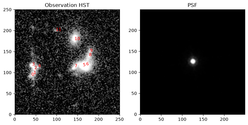
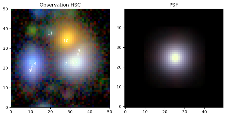
Now we display the observation contents:

norm_hst = sc2.plot.AsinhAutomaticNorm(obs_hst)
norm_hsc = sc2.plot.AsinhAutomaticNorm(obs_hsc)

sc2.plot.observation(
    obs_hst,
    norm=norm_hst,
    add_peaks=ra_dec,
    show_psf=True,
    label_kwargs={"color": "red"}
);
sc2.plot.observation(
    obs_hsc,
    norm=norm_hsc,
    add_peaks=ra_dec,
    show_psf=True
);

Define Model Frame and Stack Observations

The main difference in this tutorial is that we construct a single observation that treats the different instruments as different channels of the same (virtual) instrument, which happen to have different wavelengths and PSFs, but the same pixel grid. So, we first have to define that grid and its properties as a model frame that allows us to jointly model both data set:

model_frame = sc2.Frame.from_observations(
    observations=[obs_hst, obs_hsc],
    coverage="intersection",
)

This method defines a common area for both observations, in this case a box covering the intersection of both. Because stacking generally requires padding or truncation of the data so that it matches a common grid, it is more sensible to adopt the intersection area here. If we use coverage="union" with observations that don’t overlap well, we’ll get a stack with lots of padded zeros.

In addition to padding/truncation, we also have to resample the data if the pixel grid has different orientation, warp, or scale. Once we align these properties, the stacked observation does not require resampling during the fit, and all remaining evaluations run in parallel. The method stack_observations() performs all of these alginment steps and produces a single observations from all inputs. If any resampling has to happen (like here for the HSC data), the method automatically returns the appropriate CorrelatedObservation:

obs_stacked = sc2.stack_observations([obs_hst, obs_hsc], model_frame)
print(type(obs_stacked).__name__)

CorrelatedObservation

For more information on correlated data, see this tutorial.

Initialize Sources from a Stacked Observation

The initialization of the sources follows our general recommendation (from e.g. the quickstart guide):

with sc2.Scene(model_frame) as scene:
    infos = sc2.init.hierarchical_sources(
        obs_hst,
        K=3,
        scales=[2,3,4],
        min_area=16,
        strict=True,
        catalog=ra_dec,
        split_peaks=False,
        image_type="space"
    )
    for sinfo in infos:
        sc2.Source(sinfo.center, sinfo.spectrum, sinfo.morphology)

We choose the HST image for the initialization because it has the higher resolution and should therefore be able to better identify the position and shape of the sources. It shares the same resolution and orientation as the model frame, so the morphologies are correctly sized and oriented already. We also set split_peaks=False because the sources (especially the groups 0-4 and 7-9) definitely overlap, so we want to allow the footprints to overlap as well. And because the space-based PSF wodth is on the order of 1 pixel, the multi-scale support calculation needs to be adjusted with image_type="space".

So far, we know nothing about the sources in the HSC bands. While we could initialize these spectrum elements with zeros and let the optimization figure it the correct values, it’s much faster to use the HST-defined morphology to perform forced photometry (scarlet2.measure.forced_photometry()) in all bands, including the HSC bands. So, we should get a reasonable model across all channels of the stacked observation:

forced_spectra = sc2.measure.forced_photometry(scene, obs_stacked)
for i in range(len(scene.sources)):
    scene.sources[i] = scene.sources[i].replace("spectrum", forced_spectra[i])

We can have a quick look how the initial model looks. We use split_channels=True, so that we don’t visually merge the different observations into one (very false) color image.

sc2.plot.scene(
    scene,
    observation=obs_stacked,
    show_rendered=True,
    show_observed=True,
    show_residual=True,
    add_labels=True,
    add_boxes=True,
    box_kwargs={"edgecolor": "red", "facecolor": "none"},
    label_kwargs={"color": "red"},
    split_channels=True
);

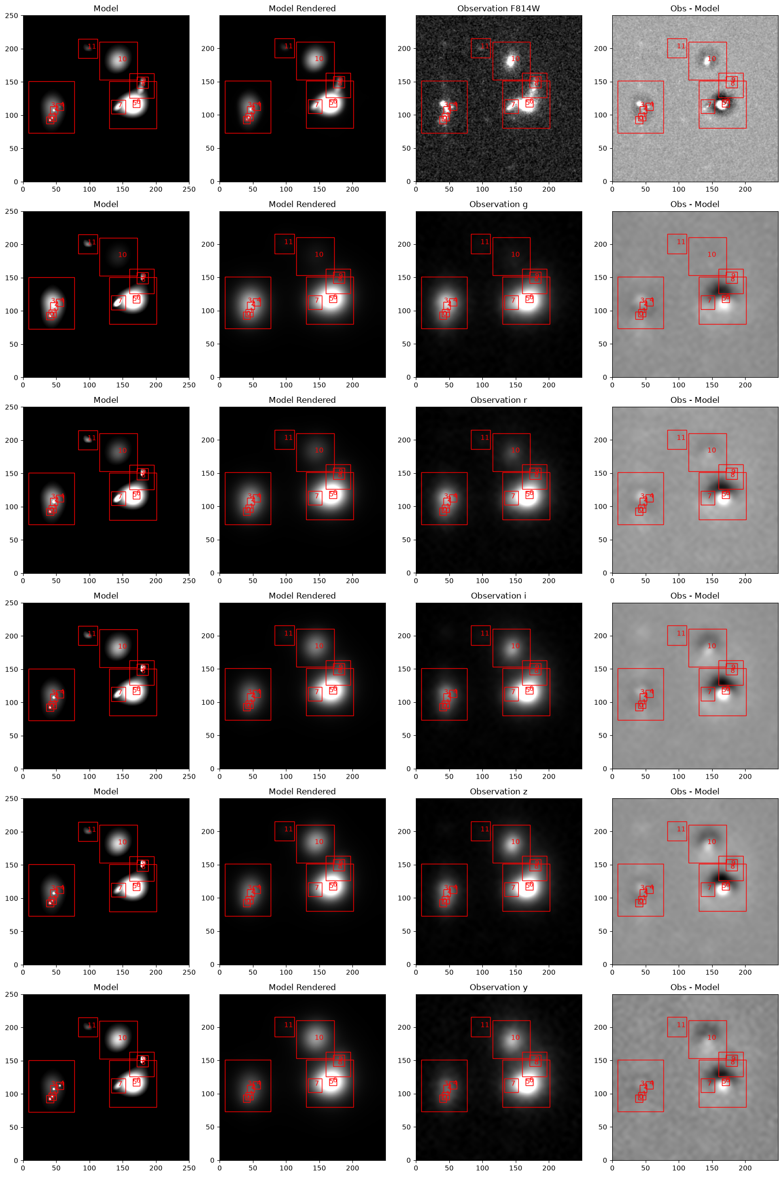
The different resolution of the different channels in this stacked observation is very apparent. But all the pixels are lined up, there is flux in all channels, and the model looks reasonable, so we’re good to go. Let’s define the fit parameters and run the fitter:

from functools import partial
from numpyro.distributions import constraints

# best step size for parameters with a relative "uncertainty":
# big/bright sources adjust more quickly
spec_step = partial(sc2.relative_step, factor=0.05)
morph_step = 0.2

with sc2.Parameters(scene):
    for i in range(len(scene.sources)):
        # because we want the spectrum parameter to be constrained,
        # we need to ensure that their initialization satisfies the constraint
        tiny = 1e-6
        spectrum = scene.sources[i].spectrum
        if (spectrum <= 0).any():
            scene.sources[i] = scene.sources[i].replace("spectrum", jnp.maximum(spectrum, tiny))
        sc2.Parameter(
            scene.sources[i].spectrum,
            name=f"spectrum:{i}",
            constraint=constraints.positive,
            stepsize=spec_step,
        )
        # same for [0,1] constrained morphology
        morph = spectrum = scene.sources[i].morphology
        if ((morph <= 0) | (morph >= 1)).any():
            scene.sources[i] = scene.sources[i].replace("morphology", jnp.clip(morph, tiny, 1-tiny))
        sc2.Parameter(
            scene.sources[i].morphology,
            name=f"morph:{i}",
            constraint=constraints.unit_interval,
            stepsize=morph_step,
        )

scene_ = scene.fit(obs_stacked, max_iter=1000, progress_bar=True)

We can now compare the model from the stacked observation to the individual observations:

sc2.plot.scene(
    scene_,
    observation=obs_hst,
    norm=norm_hst,
    show_rendered=True,
    show_observed=True,
    show_residual=True,
    add_labels=True,
    add_boxes=True,
    box_kwargs={"edgecolor": "red", "facecolor": "none"},
    label_kwargs={"color": "red"},
);
sc2.plot.scene(
    scene_,
    observation=obs_hsc,
    norm=norm_hsc,
    show_rendered=True,
    show_observed=True,
    show_residual=True,
    add_labels=True,
    add_boxes=True,
    box_kwargs={"edgecolor": "red", "facecolor": "none"},
    label_kwargs={"color": "red"},
);

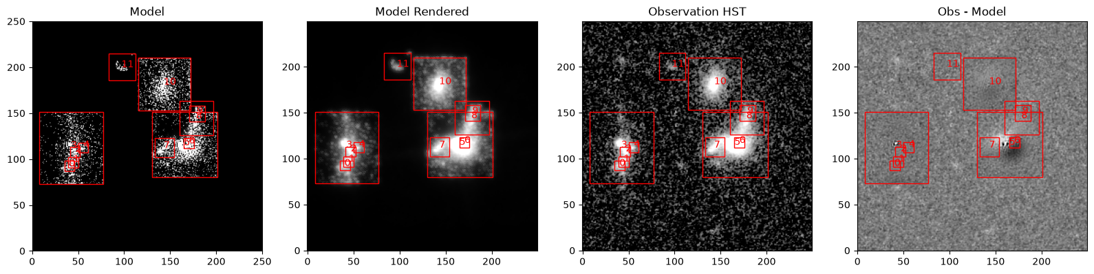
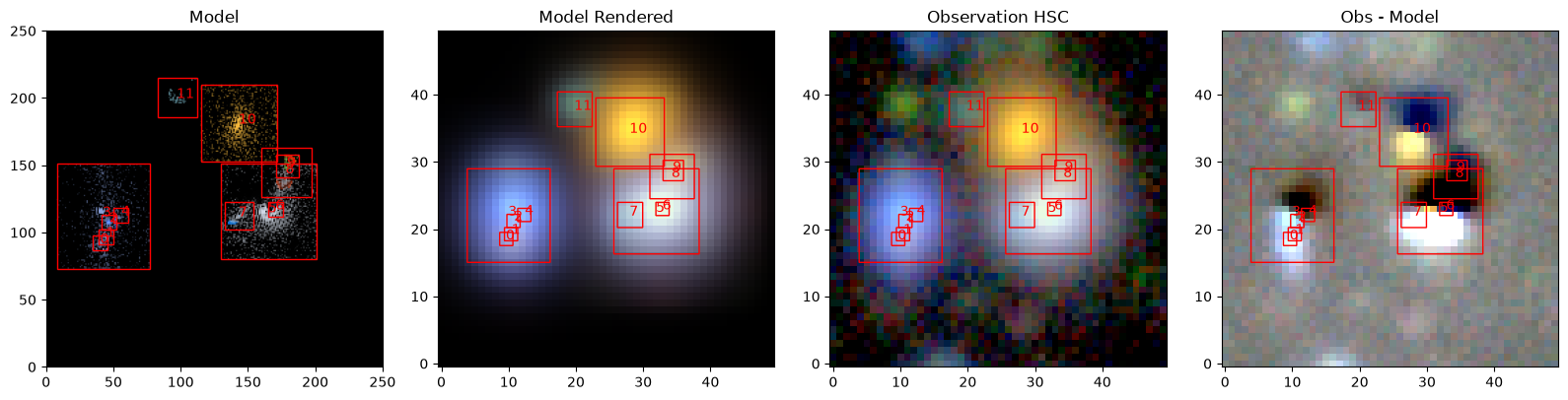
The model is pretty good, but the residuals shows pronounced dipoles. That’s is a consequence of inconsistencies of the astrometry between HST and HSC even at native resolution and stacking PSFs with different shapes. But we have a mechanism to fix that:

Fit Astrometric Offsets

The stacked observation has one renderer with a convolution being the the only transformation (which is what makes it fast). This transformation has an attribute .shift that we can define as a Parameter and refit. Originally, we parameterized the shift only for the HSC observation, which defined it as the astrometric correction wrt. the (fixed) HST observation. With a stacked observation, we can’t do that because there’s only one pixel grid for both observations. But the shift can be set as a per-channel shift. This is clearly flexible enought, but is in fact too flexible. If shifts are permitted in all channels, nothing remains to define the astrometric reference.

Tip

Define per-channel shifts with a multi-dimensional prior that has essentially zero width for at least one channel. This channel (or set of channels) then defines the astrometric reference.

# define shift parameter: unconstrained, with milli-arcsec stepsize
import astropy.units as u
import numpyro.distributions as dist

# replace the 2D shift with a (C,2) shift
C = obs_stacked.frame.C
shift = jnp.zeros((C, 2))
object.__setattr__(obs_stacked.renderer[-1], "shift", shift)

ref_channel = 0
with sc2.Parameters(obs_stacked):
    # define a Gaussian prior with zero mean and narrow width in ref_channel
    scale = jnp.ones((C, 2))
    scale = scale.at[ref_channel].set(1e-3)
    scale = 0.1 * scale * u.arcsec
    prior = dist.Normal(shift, scale=scale).to_event(2) # last 2 dims are per-event

    # declare new shift as parameter
    sc2.Parameter(obs_stacked.renderer[-1].shift, name="shift", prior=prior, stepsize=1e-3 * u.arcsec)

# the more flexible fitter optimizes scene and observation and returns both
scene_, obs_stacked_ = sc2.infer.fit(scene_, obs_stacked, e_rel=1e-4, max_iter=1000)

# get the astrometry shift
shift = obs_stacked_.get("shift")
print("\nShift per channel in model pixels:")
print(shift)

Shift per channel in model pixels:
[[ 5.5478008e-06  4.0376199e-06]
 [-1.3682866e+00  6.2238097e-01]
 [-1.3363540e+00  2.3455234e-01]
 [-1.3380040e+00  2.4820605e-01]
 [-1.2052517e+00  2.6474398e-01]
 [-1.2252852e+00  2.8635213e-01]]

Now we have the shift in every channel as an independent variable, with the first channel clamped down to almost zero. That can be appropriate, in particular if the PSFs in HSC are not well-aligned internally, but usually the problem stems from differences in astrometric fitting and PSF modeling between instruments or surveys. Allowing every channel to have its own shift may be overkill and just pick up spurious shifts from noise or complex wavelength-dependent morphologies.

We could keep the above and average all of the HSC-channel shifts, but the best option is to create a shift per observation, where the channels of the original observations share the shift parameter. The following achieves this task:

class ShiftPerObservation(sc2.Module):
    """Create multi-channel shift from 2D shifts per observation"""
    shifts: tuple
    channel_index: tuple
    C: int

    def __init__(self, observations, frame):
        if not isinstance(observations, (list, tuple)):
            observations = (observations,)
        self.shifts = tuple(jnp.zeros((2,)) for obs in observations)
        self.channel_index = tuple(jnp.array([frame.channels.index(c) for c in obs.frame.channels]) for obs in observations)
        self.C = frame.C
    def __call__(self):
        shift = jnp.zeros((C, 2))
        for i,c in enumerate(self.channel_index):
            shift = shift.at[c].set(self.shifts[i])
        return shift

# replace the 2D shift with a per-observation shift model
shifted_obs = (obs_hsc,) # only allow HSC obs to shift
per_obs_shift = ShiftPerObservation(shifted_obs, obs_stacked.frame)
object.__setattr__(obs_stacked.renderer[-1], "shift", per_obs_shift)

with sc2.Parameters(obs_stacked):
    # define a Gaussian prior for shift(s)
    scale = 0.1 * jnp.ones((2,)) * u.arcsec
    prior = dist.Normal(jnp.zeros((2,)), scale=scale).to_event(1) # last dim are per-event

    # declare new shift(s) as parameter(s)
    for shift,obs in zip(per_obs_shift.shifts, shifted_obs):
        sc2.Parameter(shift, name=f"shift_{obs.name}", prior=prior, stepsize=1e-3 * u.arcsec)

# let's fit again..
scene_, obs_stacked_ = sc2.infer.fit(scene_, obs_stacked, e_rel=1e-4, max_iter=1000)

# get the astrometry shift by evaluating the shift model
shift = obs_stacked_.renderer[-1].shift()
print("\nShift per channel in model pixels:")
print(shift)

# now get the actual free parameter
hsc_shift = obs_stacked_.get("shift_HSC")
print(f"Shift of HSC in model pixels: {hsc_shift}")

Shift per channel in model pixels:
[[ 0.          0.        ]
 [-1.4953393   0.25835118]
 [-1.4953393   0.25835118]
 [-1.4953393   0.25835118]
 [-1.4953393   0.25835118]
 [-1.4953393   0.25835118]]
Shift of HSC in model pixels: [-1.4953393   0.25835118]

So, all HSC channels share the same shift, and the HST observation didn’t shift at all: perfect! To evaluate the model in the native pixel grid of HSC, we need to convert the astrometric offset we have just determined from the model grid to the HSC grid:

# get the Jacobian transform between resampled model and native HSC frame
jacobian, _ = sc2.frame.get_relative_jacobian_shift(obs_stacked.frame, obs_hsc.frame)
shift_native = jacobian @ hsc_shift
print(f"Shift in native HSC pixels: {shift_native}")

# force the renderer to use optimized value for shift
object.__setattr__(obs_hsc.renderer[-1], "shift", shift_native)

Shift in native HSC pixels: [-0.26702484  0.04613414]

sc2.plot.scene(
    scene_,
    observation=obs_hst,
    show_rendered=True,
    show_observed=True,
    show_residual=True,
    add_labels=True,
    add_boxes=True,
    norm=norm_hst,
    box_kwargs={"edgecolor": "red", "facecolor": "none"},
    label_kwargs={"color": "red"},
)
sc2.plot.scene(
    scene_,
    observation=obs_hsc,
    show_rendered=True,
    show_observed=True,
    show_residual=True,
    add_labels=True,
    add_boxes=True,
    norm=norm_hsc,
);

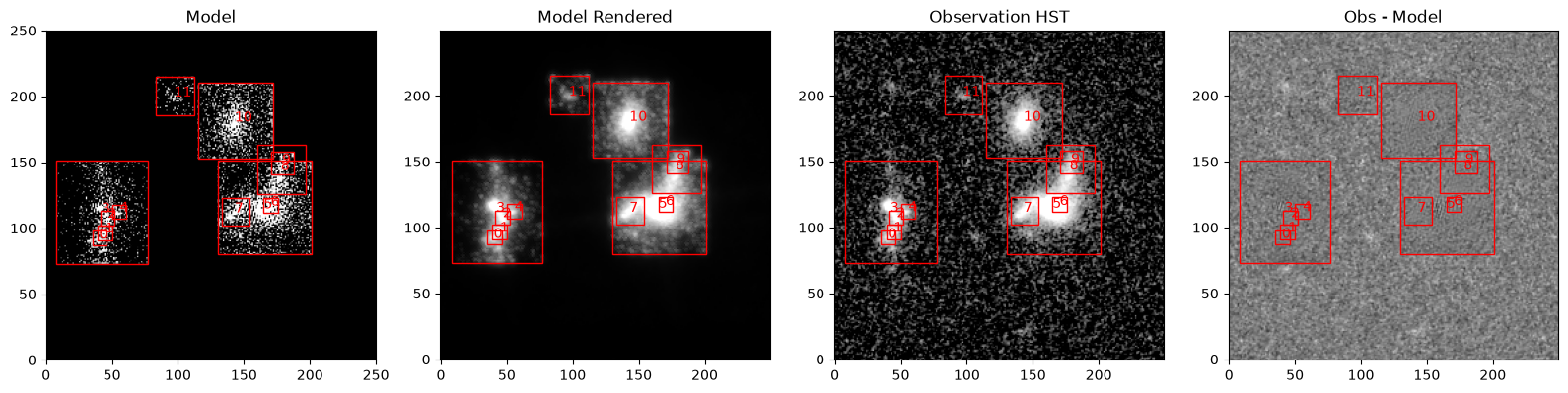
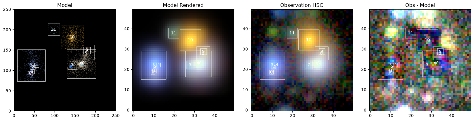
Look Ma, no dipoles! We can thus concentrate on modeling sources…